
Step 6: Multiple Regression
- Multiple regression puts several explanatory variables in one equation, \( y = \beta_0 + \beta_1 x_1 + \cdots + \beta_k x_k + u \). Each slope is a partial effect: the change in \( y \) when one regressor rises by one unit and the others are held fixed.
- OLS still minimises the sum of squared residuals. Each slope uses only the part of its regressor that the other regressors cannot predict (the Frisch–Waugh, or partialling-out, result).
- \( R^2 \) can never fall when you add a variable. Adjusted \( R^2 \) charges for each extra regressor and rises only if the new variable has \( |t| > 1 \).
- Leaving out a relevant variable \( x_2 \) biases the coefficient on \( x_1 \) by \( \beta_2\delta_1 \): its effect on \( y \) times its slope on \( x_1 \). Both must be non-zero for a problem.
- Exam point: \( \operatorname{Var}(\hat\beta_j) = \sigma^2 / [\text{SST}_j(1-R_j^2)] \). Correlation among regressors costs precision, not unbiasedness.
- How to read each coefficient in a multiple regression as a ceteris paribus effect, including when a variable also enters as a square.
- What OLS actually does with several regressors, and why a coefficient can collapse once a control is added.
- How to use \( R^2 \) and adjusted \( R^2 \), and why neither tells you whether a variable belongs in the model.
- The assumptions MLR.1 to MLR.5, perfect collinearity, and the Gauss–Markov theorem.
- How to derive, sign and check omitted variable bias, and what drives the standard error of each slope.
Why one regressor is rarely enough
A simple regression of \( y \) on one \( x \) compares people, firms or houses that differ in that one variable. It lets everything else vary however it happens to vary. Workers with more schooling may also be younger, more often urban or more often in a union. Houses with more bedrooms are also bigger. The simple regression credits all of these differences to the single variable you included.
Multiple regression fixes this by moving other factors out of the error term and into the equation. Take the wage equation from Step 3 and add experience:
Now \( \beta_1 \) is the effect of a year of education holding experience fixed, and \( \beta_2 \) is the effect of a year of experience holding education fixed. We no longer need education to be unrelated to experience. The model allows the two to move together and separates their effects.
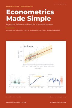 Chapter 6 of Econometrics Made Simple covers this in full: OLS with several regressors, partialling out, omitted variable bias and the Gauss–Markov theorem, with Python, R and Stata code for every result.Get the textbook · $15
A laboratory scientist holds other factors fixed by design. An economist cannot assign people their schooling, but multiple regression compares them as if their other included characteristics were the same. It does this statistically, and only for the variables you include. Anything still in \( u \) is not held fixed.
The model with \( k \) regressors
The general model has \( k \) explanatory variables and \( k+1 \) unknown parameters (the intercept plus \( k \) slopes):
The second expression says the effects add up when several variables change at once. “Linear” means linear in the \( \beta \)s, not in the variables. A regressor can be a square or a log. A standard wage equation includes experience and experience squared:
Here \( \beta_2 \) alone is not “the effect of experience”, because exper and exper² cannot change independently. The effect depends on how much experience the worker already has. Step 8 treats quadratics fully.
What OLS does with several regressors
OLS works exactly as in simple regression. It chooses \( \hat\beta_0, \dots, \hat\beta_k \) to make the sum of squared residuals as small as possible. Setting each derivative to zero gives \( k+1 \) first-order conditions:
In words: the residuals average to zero and have zero sample covariance with every regressor. If any linear relationship were left between the residuals and an \( x \), a different coefficient would fit better. A computer solves these equations instantly. You do not need matrix algebra to use or interpret the results.
Partialling out: what “holding fixed” means
The clearest way to see what a multiple-regression slope measures is the Frisch–Waugh (or Frisch–Waugh–Lovell) theorem. The coefficient on educ in the two-regressor wage model can be found in two steps:
With the 1,000 workers in wages.csv, the companion data for Econometrics Made Simple, both routes give 0.104092, identical to six decimal places (Chapter 6). The slope uses only the variation in schooling that is not shared with experience. That is precisely what “holding experience fixed” means. With more regressors the idea is the same: regress \( x_j \) on all the other \( x \)s, keep the residuals, and regress \( y \) on them.
Worked example: four wage models
Good practice is to start small and add variables in groups, watching how the coefficient you care about responds. Chapter 6 of the book estimates four models for log(wage): (1) education only; (2) adding experience; (3) adding exper² and tenure; (4) adding dummies for female, married, urban and union. Standard errors are in brackets.
| Variable | (1) | (2) | (3) | (4) |
|---|---|---|---|---|
| educ | 0.1026 (0.0081) | 0.1041 (0.0079) | 0.1042 (0.0077) | 0.1054 (0.0075) |
| exper | 0.0120 (0.0015) | 0.0303 (0.0057) | 0.0294 (0.0055) | |
| exper² | −0.00058 (0.00012) | −0.00056 (0.00012) | ||
| tenure | 0.0162 (0.0032) | 0.0152 (0.0031) | ||
| female | −0.1550 (0.0279) | |||
| married / urban / union | 0.0776 / 0.1080 / 0.1453 | |||
| \( R^2 \) | 0.1387 | 0.1885 | 0.2268 | 0.2736 |
| Adjusted \( R^2 \) | 0.1378 | 0.1868 | 0.2237 | 0.2677 |
Using Model (4), interpret the coefficients on educ, tenure, female and urban.
Every interpretation ends with the ceteris paribus clause. Without it the number has no meaning, because the coefficient on education “holding experience fixed” is a different quantity from the coefficient “holding age fixed”.
In Model (3) the experience terms are \( 0.0303\,\text{exper} – 0.000576\,\text{exper}^2 \). Find the effect of one more year of experience at 10 and at 20 years, and the experience at which predicted wages stop rising.
Experience pays most early in a career. Few workers in the sample have much more than 26 years, so the turn-down beyond that point is estimated less reliably than the rise.
Why the education coefficient hardly moves
Across the four models the education coefficient goes from 0.1026 to 0.1041, 0.1042 and 0.1054. Seven extra variables, several highly significant, barely change it. The reason is that education is almost unrelated to the variables added: the correlation between educ and exper in this sample is only −0.025. A coefficient changes when you add a control only if the control both affects \( y \) and is correlated with the regressor. The omitted variable bias formula below turns this into arithmetic.
Worked example: why bedrooms stop mattering
The house data tell the opposite story. Regressed on its own, the number of bedrooms looks like a powerful driver of price. Chapter 6 runs the comparison on the 500 sales in houses.csv (prices in $000):
Alone, the bedrooms coefficient is 66.12 (\( t = 17.2 \)). After adding sqft, age and dist_cbd it is 7.28 (\( t = 1.56 \), \( p = 0.119 \)). Explain the change.
About $66,000 per bedroom becomes about $7,300, and it is no longer significantly different from zero.
Goodness of fit: \( R^2 \) and adjusted \( R^2 \)
The decomposition from simple regression carries over: \( \text{SST} = \text{SSE} + \text{SSR} \) and \( R^2 = 1 – \text{SSR}/\text{SST} \). \( R^2 \) is the share of the variation in \( y \) explained by all the regressors together. In the wage table it rises from 0.1387 to 0.2736.
Look at that row again: 0.1387, 0.1885, 0.2268, 0.2736. It only goes up, and that is not luck. When you add \( x_{k+1} \), OLS could set its coefficient to zero and reproduce the old SSR. It picks the smallest SSR available, so the new SSR is the same or lower, and \( R^2 \) cannot fall. Even a variable unrelated to \( y \) nudges \( R^2 \) up by fitting chance patterns. Adding parents’ education to Model (2), a variable with no direct effect on wages in these simulated data, still raises \( R^2 \) from 0.1885 to 0.1894.
Adjusted \( R^2 \) replaces sums of squares with variance estimates. Adding a regressor lowers SSR (which helps) but also lowers \( n-k-1 \) (which hurts), so \( \bar R^2 \) can fall. It rises when a single variable is added if and only if that variable’s \( |t| \) is greater than 1. Parents’ education has \( t = -1.09 \), so \( \bar R^2 \) creeps up from 0.1868 to 0.1870.
Model (4) has \( R^2 = 0.2736 \), \( n = 1{,}000 \) and \( k = 8 \). Compute \( \bar R^2 \). What would it be with the same \( R^2 \) but only 40 observations?
With 1,000 observations the penalty for eight regressors is tiny. With 40 it wipes out most of the fit.
For a full comparison of the two measures, with more examples, see our post R-Squared vs Adjusted R-Squared: What They Mean and When to Use Each.
The assumptions, collinearity and Gauss–Markov
To say how OLS behaves across repeated samples, extend the simple-regression assumptions of Step 4:
| Assumption | Statement |
|---|---|
| MLR.1 | Linear in parameters: \( y = \beta_0 + \beta_1x_1 + \cdots + \beta_kx_k + u \). |
| MLR.2 | Random sample of \( n \) observations from that population. |
| MLR.3 | No perfect collinearity: no regressor is constant, and none is an exact linear combination of the others. |
| MLR.4 | Zero conditional mean: \( E(u \mid x_1,\dots,x_k) = 0 \). |
| MLR.5 | Homoskedasticity: \( \operatorname{Var}(u \mid x_1,\dots,x_k) = \sigma^2 \). |
Under MLR.1–MLR.4, OLS is unbiased: \( E(\hat\beta_j) = \beta_j \). MLR.4 does the real work, and it is more plausible than in simple regression, because every variable moved from \( u \) into the equation is one fewer source of trouble. Adding MLR.5 gives the Gauss–Markov theorem: OLS is the best linear unbiased estimator (BLUE), the one with the smallest variance among estimators that are linear in \( y \) and unbiased.
Perfect collinearity: a real example
MLR.3 fails when one regressor is an exact linear function of others: income in dollars and in thousands of dollars; both female and male \( = 1-\text{female} \) with an intercept (the dummy-variable trap of Step 9); or age, education and experience when experience is computed as age − educ − 6. That last case is built into wages.csv: all 1,000 rows satisfy the identity, and a regression of exper on age and educ has \( R^2 = 1 \). Software drops one variable.
Dropping a variable changes what the others mean. With educ and age in the model, the education coefficient is 0.0921, not 0.1041. Holding age fixed, a year more at school is a year less of work, so the coefficient is the return to schooling net of lost experience: \( 0.1041 – 0.0120 = 0.0921 \). Both models have \( R^2 = 0.1885 \). They answer different questions.
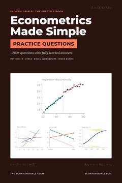 Partial effects and omitted variable bias come up in almost every econometrics exam. The Practice Questions book has over 1,150 questions, every one with a worked answer.Get 1,150+ questions · $9
Omitted variable bias
Suppose the true model is \( y = \beta_0 + \beta_1x_1 + \beta_2x_2 + u \), but you regress \( y \) on \( x_1 \) alone and get the slope \( \tilde\beta_1 \). Let \( \tilde\delta_1 \) be the slope from regressing \( x_2 \) on \( x_1 \). Then, in any sample, exactly,
The bias is zero in exactly two cases: the omitted variable does not affect \( y \) (\( \beta_2 = 0 \)), or it is uncorrelated with the included regressor (\( \delta_1 = 0 \)). The sign follows from the two signs:
| \( \operatorname{Corr}(x_1,x_2) > 0 \) | \( \operatorname{Corr}(x_1,x_2) < 0 \) | |
|---|---|---|
| \( \beta_2 > 0 \) | Positive bias (overstates \( \beta_1 \)) | Negative bias |
| \( \beta_2 < 0 \) | Negative bias | Positive bias |
Check the identity for the house data. In the regression of price on sqft and bedrooms, the coefficients are 0.1332 on sqft and 5.4214 on bedrooms. The slope from regressing sqft on bedrooms is 455.7 square feet per bedroom. What is the simple-regression slope on bedrooms?
Almost all of the apparent $66,000 value of a bedroom is the value of the extra 456 square feet that comes with it.
Every wage model above leaves out ability, because it is not measured. Predict the direction of the bias in the education coefficient.
Because the companion data are simulated, the book can check: the true return built into wages.csv is 0.085, while Model (4) estimates 0.1054, about two percentage points too high. Adding observed controls did not remove the bias, because none of them is a good stand-in for ability. Step 13 uses an instrument to get closer.
The same identity explains the stable education coefficient. Omitting experience, the long regression gives 0.10409 on educ and 0.01197 on exper, and the slope of exper on educ is −0.12595. So \( 0.10409 + 0.01197 \times (-0.12595) = 0.10258 \), the short-regression slope. The bias is only −0.0015 because \( \tilde\delta_1 \) is tiny. Omitting tenure from a regression on experience is different: tenure raises wages (0.01598) and rises strongly with experience (0.40224 years per year), so the experience coefficient more than doubles, from 0.00505 to 0.01147. For a step-by-step method to predict the sign before you run anything, read Omitted Variable Bias: How to Predict the Direction.
The precision of each slope
Unbiasedness says the estimates are right on average. Their variance says how far a typical estimate lies from the truth. Under MLR.1–MLR.5,
where \( \text{SST}_j \) is the total variation in \( x_j \) and \( R_j^2 \) is the \( R^2 \) from regressing \( x_j \) on the other regressors. Three things set the precision: the noise in \( y \) (\( \sigma^2 \)); the spread of \( x_j \), which grows with the sample size; and how well the other regressors predict \( x_j \). The factor \( 1/(1-R_j^2) \) is the variance inflation factor.
For educ in Model (2): \( \hat\sigma^2 = 0.21470 \), \( \text{SST}_{\text{educ}} = 3476.1 \) and \( R_j^2 = 0.00060 \). Rebuild the standard error.
Adding parents’ education, which is correlated with own education, raises \( R_j^2 \) to 0.1391 and the standard error to 0.00847, while the coefficient moves only from 0.1041 to 0.1075.
This gives the key trade-off. Including an irrelevant variable causes no bias, but if it is correlated with \( x_j \) it raises the variance. Omitting a relevant variable that is correlated with \( x_j \) causes bias that more data will not cure. In large samples the bias is usually the bigger danger, so researchers include a control when theory says it affects \( y \) and it is plausibly correlated with the variable of interest. The exception, a control that is itself an outcome of that variable, is the “bad control” of Step 10.
Practise: 6 questions
Try each one on paper first, then check the worked answer.
EasyQ1. A regression of house prices ($000) gives \( \widehat{\text{price}} = 40 + 0.12\,\text{sqft} + 9\,\text{bedrooms} – 1.5\,\text{age} \). (a) Interpret 0.12. (b) By how much does the predicted price change if floor area rises by 250 sq ft with bedrooms and age fixed? (c) Predict the price of a 1,800 sq ft, 3-bedroom, 20-year-old house. Show worked answer
(b) \( \Delta\widehat{\text{price}} = 0.12 \times 250 = 30 \): $30,000 higher.
(c) \( 40 + 0.12(1800) + 9(3) – 1.5(20) = 40 + 216 + 27 – 30 = 253 \): about $253,000.
EasyQ2. A model with \( k = 4 \) regressors and \( n = 61 \) observations has \( R^2 = 0.40 \). Compute adjusted \( R^2 \). Show worked answer
\( = 1 – 0.6429 = 0.357 \).
The penalty is noticeable because \( n \) is small relative to \( k \).
MediumQ3. Across shops, monthly sales ($000) are regressed on advertising spending (\( x_1 \), $000) and the number of sales staff (\( x_2 \)). The long regression gives \( \hat\beta_1 = 0.50 \) and \( \hat\beta_2 = 2.0 \). Regressing staff on advertising gives a slope of 0.30. (a) What slope on advertising would a regression of sales on advertising alone give? (b) Explain the direction of the bias. Show worked answer
(b) Staff raise sales (\( \beta_2 > 0 \)) and shops that advertise more also employ more staff (\( \delta_1 > 0 \)). The bias \( \beta_2\delta_1 = 0.60 \) is positive: the short regression credits advertising with the effect of the extra staff and more than doubles its apparent effect.
MediumQ4. In a regression, \( \hat\sigma^2 = 0.25 \), \( \text{SST}_j = 400 \) and \( R_j^2 = 0.75 \). (a) Compute \( \operatorname{se}(\hat\beta_j) \) and the VIF. (b) What would the standard error be if \( x_j \) were uncorrelated with the other regressors? Show worked answer
(b) With \( R_j^2 = 0 \): \( \sqrt{0.25/400} = 0.025 \).
The standard error doubles, by the factor \( \sqrt{\text{VIF}} = \sqrt{4} = 2 \).
MediumQ5. A wage equation contains \( 0.045\,\text{exper} – 0.0009\,\text{exper}^2 \) (the dependent variable is log wage). Find the partial effect of experience at 10 years, and the turning point. Show worked answer
At 10 years: \( 0.045 – 0.018 = 0.027 \), so one more year raises the wage by about 2.7%, other regressors fixed.
Turning point: \( 0.045 = 0.0018\,\text{exper} \), so \( \text{exper} = 25 \) years.
The coefficient 0.045 alone is the effect only at zero experience.
ExamQ6. A researcher models household electricity use (kWh per month) across 800 homes. (a) She first tries regressors income ($000), number of adults, number of children and household size, where size = adults + children. Explain what goes wrong. [2] (b) She settles on two models. Electricity on income alone gives a slope of 3.2. Electricity on income and household size gives 2.0 on income and 40 on size. Find the slope from regressing household size on income. [3] (c) State the direction of the bias in the first model and explain it in words. [2] Show worked answer
(b) Use \( \tilde\beta_1 = \hat\beta_1 + \hat\beta_2\tilde\delta_1 \): \( 3.2 = 2.0 + 40\,\tilde\delta_1 \). [M1]
\( \tilde\delta_1 = 1.2/40 = 0.03 \). [A1]
Richer households have, on average, 0.03 more members per $1,000 of income. [A1]
(c) The bias is \( 40 \times 0.03 = +1.2 \): upward. [B1] Bigger households use more electricity and are richer on average, so the income-only slope credits income with part of the effect of household size. [B1]
Total: 7 marks.
Check yourself
1. In \( y = \beta_0 + \beta_1x_1 + \beta_2x_2 + u \), what does \( \beta_2 \) measure?
2. You add a fifth regressor to a model with four. Which is always true?
3. The omitted variable raises \( y \) and is negatively correlated with \( x_1 \). The short-regression slope on \( x_1 \) is
Your score: 0 out of 3
The short version
- Each slope in a multiple regression is a partial effect: the change in \( y \) when one regressor rises by one unit and the others are held fixed. If a variable also enters squared, its effect is \( \beta_2 + 2\beta_3x \).
- OLS makes the residuals sum to zero and uncorrelated with every regressor. By Frisch–Waugh, each slope uses only the variation in its regressor not explained by the others.
- Controls change a coefficient only if they affect \( y \) and are correlated with the regressor: the return to education stays at 0.10–0.11, while the bedrooms coefficient falls from 66.1 to 7.3 once floor area is held fixed.
- \( R^2 \) never falls when a regressor is added; \( \bar R^2 = 1-(1-R^2)(n-1)/(n-k-1) \) rises only if the new variable has \( |t| > 1 \).
- Omitting \( x_2 \) biases the coefficient on \( x_1 \) by \( \beta_2\delta_1 \). Omitted ability biases the return to schooling upwards: 0.105 against a true 0.085 in the book’s simulated data.
- \( \operatorname{Var}(\hat\beta_j) = \sigma^2/[\text{SST}_j(1-R_j^2)] \). Irrelevant variables cost precision; omitted relevant ones cause bias. Under MLR.1–MLR.5, OLS is BLUE.
- Chapter 6 of Econometrics Made Simple has the full derivations, Python, R and Stata code for every result, and a full set of exercises with answers.
 Work through multiple regression with the full chapter and hundreds of graded questions. Get the textbook and the practice book together for $19 (was $24).Both books · $19
Studying more than one subject? The Complete Book Bundle includes every Economics, Statistics, Mathematics and Econometrics book we publish.
Further reading on EconTutorials
Related in-depth articles from our blog, and the neighbouring steps:
- R-Squared vs Adjusted R-Squared: What They Mean and When to Use Each
- Omitted Variable Bias: How to Predict the Direction Before You Run the Regression
- Ordinary Least Squares (OLS): Derivation, Assumptions, and Why Omitted Variable Bias Ruins Everything
- How to Read Regression Output: Every Number Explained
- Previous step: Step 5: Inference: t-Tests and Confidence Intervals
- Next step: Step 7: F-Tests and Joint Hypotheses