Econometrics guide, Unit 2, step 10 of 20Previous step Next step

Step 10: Model Specification and Multicollinearity

By the EconTutorials team. 15-minute read with 6 practice questions.

Course matchIntroductory econometrics: specification and data issues · Wooldridge Ch. 3 and 9 · Stock & Watson Ch. 9

In 30 seconds

A specification error is a wrong choice of variables, functional form, measurement or sample. Some cause bias (omitted variables, bad controls, wrong form, error in $ x $, selection on $ y $); others only cost precision.
Multicollinearity (high but imperfect correlation among regressors) causes no bias. It inflates variances by $ \text{VIF}_j = 1/(1-R_j^2) $. Never “fix” it by dropping a relevant variable.
A bad control is an outcome of the variable you care about; holding it fixed removes part of the effect you want.
RESET adds $ \hat y^2 $ and $ \hat y^3 $ to test functional form. Classical measurement error in $ x $ biases the slope towards zero by the reliability ratio.
Exam point: find influential points with leverage, studentised residuals and Cook’s distance, but correct only genuine errors. Never delete data because it is inconvenient.

Video lesson coming soonA short animated lesson for this step will appear here.

What you will learn

The main types of specification error and which ones bias your estimates.
How to recognise multicollinearity, compute VIFs, and what to do (and not do) about it.
How to choose controls, spot bad controls and judge a proxy variable.
How to run Ramsey’s RESET, the $ J $ test and the AIC and BIC.
What measurement error, missing data and selected samples do to OLS, and how to handle influential observations.

What is a specification error?

Every regression rests on choices: which variables, in what form, measured how, on which observations. Each can be wrong, and none shows up as an error message. The software reports neat coefficients and small standard errors whatever you feed it. This step is about the checks that stand between a regression and a believable result.

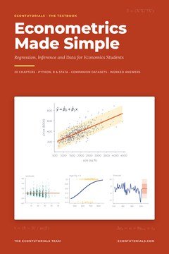Key termA specification error is any mistake in the choice of the estimated model: which variables are included, the functional form, how variables are measured, or which observations are used. Errors that cost precision make confidence intervals wider but keep them honest. Errors that cause bias make the answer wrong in a way that more data will not fix.

Chapter 10 of Econometrics Made Simple covers this in full: multicollinearity and VIFs, bad controls, proxies, RESET, measurement error, selected samples and influence diagnostics, ending with a project checklist.Get the textbook · $15

Specification error	Consequence for OLS	How to detect or avoid it
Omitted relevant variable	Bias if correlated with an included $ x $	Theory; sign the bias; proxies
Irrelevant variable included	No bias; larger variance	$ t $ and $ F $ tests; theory
Bad control (an outcome of $ x $)	Bias: removes part of the effect	Ask what causes what
High multicollinearity	No bias; large variances	VIFs; joint tests
Wrong functional form	Bias in the partial effects	RESET; plots; $ J $ test
Measurement error in $ x $	Bias towards zero	Better data; instruments
Measurement error in $ y $	No bias; larger variance	Better data
Sample selected on $ y $	Bias	Know how the sample was drawn
Influential observations	Results driven by a few points	Leverage; Cook’s distance

Multicollinearity

Step 6 met perfect collinearity, an exact linear relationship such as exper = age − educ − 6, which breaks MLR.3. Multicollinearity is different: one regressor is highly, but not perfectly, correlated with a combination of the others. It breaks no assumption. OLS is still unbiased and BLUE. It makes the affected coefficients imprecise, because little independent variation is left to estimate each separate effect.

\[ \operatorname{Var}(\hat\beta_j) = \frac{\sigma^2}{\text{SST}_j} \times \underbrace{\frac{1}{1-R_j^2}}_{\text{VIF}_j}, \qquad \text{tolerance}_j = 1 – R_j^2 = \frac{1}{\text{VIF}_j}. \]

The standard error is inflated by $ \sqrt{\text{VIF}_j} $ compared with a regressor uncorrelated with the others. Inflation grows slowly: to multiply a standard error by 10 needs VIF = 100, that is $ R_j^2 = 0.99 $.

Worked example

Chapter 10 of Econometrics Made Simple regresses house price on sqft, lot, bedrooms, bathrooms, age, dist_cbd and pool (500 sales). The other regressors explain $ R_j^2 = 0.771 $ of the variation in sqft. Compute its VIF, tolerance and standard-error inflation.

Step 1VIF $ = 1/(1-0.771) = 4.367 $.

Step 2Tolerance $ = 1 – 0.771 = 0.229 $.

Step 3Standard-error inflation: $ \sqrt{4.367} = 2.09 $.

The four size measures overlap heavily. Age, distance and pool, with VIFs of about 1.01 to 1.02, are almost unrelated to size, so their coefficients are as precise as the sample allows.

Variance inflation factors in the house-price regression VIF = 1/(1 − Rⱼ²)

Figure 1. VIFs for price regressed on sqft, lot, bedrooms, bathrooms, age, dist_cbd and pool (500 sales). The four size measures overlap heavily: the others explain 77.1% of the variation in floor area, so its standard error is √4.367 = 2.09 times what it would otherwise be. Age, distance and pool are almost unrelated to size (VIF ≈ 1). Econometrics Made Simple, Chapter 10.

The symptoms

Multicollinearity has three classic symptoms, all from one cause: the data cannot tell the correlated variables apart. (1) Large standard errors on the correlated variables, often with odd signs. (2) Joint but not individual significance. (3) Unstable coefficients across samples. It is above all a small-sample problem, because $ \text{SST}_j $ grows with $ n $.

The book shows this with the first 30 sales only. Floor area has $ p = 0.072 $, bedrooms $ p = 0.920 $ (with a standard error ten times its coefficient) and bathrooms $ p = 0.118 $. A careless reader would say size does not matter. Yet the $ F $ test that all four size variables are zero gives $ F = 20.21 $, $ p = 2.9 \times 10^{-7} $. Across neighbourhoods, the sqft coefficient stays between 0.107 and 0.135, while the bedrooms coefficient swings from −5.809 to 13.616.

What to do, and what not to do

First ask whether there is a problem at all. If the coefficient you care about is precise enough, collinearity among the other regressors does not matter. When it does matter: get more data; test the collinear group jointly (Step 7); combine the variables into an index; ask a question the data can answer, such as the value of a bundle of extra space and an extra bedroom; or centre polynomial terms to reduce the collinearity between $ x $ and $ x^2 $.

Worked example

In the full house regression the bedrooms coefficient is 4.680 (se 5.422), not significant. A student drops sqft “to fix the multicollinearity”. The bedrooms coefficient becomes 40.877 (se 5.194), with $ t $ near 8. What went wrong?

Step 1sqft affects price and is strongly correlated with bedrooms, so dropping it creates omitted variable bias.

Step 2Bedrooms now carries the value of the floor area that comes with it; the lot coefficient also jumps, from 0.001 to 0.017.

Step 3The standard error barely moved (5.422 to 5.194). Dropping sqft bought almost no precision and a large bias.

This is the precision problem swapped for a bias problem. For the difference between the two kinds of collinearity, see Difference between Perfect and Imperfect Multicollinearity.

Common mistakeTreating a VIF above 10 (or 5) as a test that the model is wrong. These cut-offs are conventions, not theorems. A VIF of 12 on a variable with $ t = 8 $ is no problem, and a VIF of 2 can matter in a sample of 30. What matters is whether the coefficients you care about are precise enough to answer your question.

Exam tipAsked “what would you do about multicollinearity?”, give a three-part answer: OLS is still unbiased and it matters only if the key coefficients are too imprecise; remedies are more data, joint tests and combining variables; and dropping a relevant variable causes omitted variable bias.

Which controls? Bad controls and proxies

Omitting a relevant variable biases the coefficient on $ x_1 $ by $ \beta_2\delta_1 $. Including an irrelevant one costs only precision: adding parents’ education to the wage equation raised the standard error of the education coefficient from 0.00786 to 0.00847. So when a variable is plausibly relevant and correlated with the regressor of interest, it usually belongs in. There is one important exception.

Key termA bad control is a variable that is itself an outcome of the regressor of interest. Holding it fixed removes the part of the effect that works through it. Controls should be determined before the variable of interest, or at least not be affected by it.

Controlling for occupation when estimating the return to education compares two accountants with different schooling and leaves out the main channel: better jobs. The same applies to the gender pay gap. The book simulates 20,000 workers in which being female lowers the log wage by 0.10 directly and a high-paying job raises it by 0.40. Half of men (50.6%) but a quarter of women (24.9%) hold such jobs. Without the job variable the gap is −0.2043: about −0.10 directly plus $ 0.40 \times (0.249 – 0.506) = -0.103 $ through jobs. Adding the job dummy gives −0.1032, the direct effect only. Both are correct; they answer different questions.

Proxy variables

A proxy is an observed variable included in place of an unobserved one, such as an IQ score for ability. It works only if, once the proxy is held fixed, the rest of the omitted factor is unrelated to the regressor. In practice a proxy usually reduces the bias rather than removing it. In the book’s simulation with a true return of 0.08, omitting ability gives 0.1065, adding a noisy test score gives 0.0857, and adding true ability gives 0.0773. Parents’ education, by contrast, moves the coefficient the wrong way (0.1048 to 0.1078), because in these data it shifts schooling but is unrelated to ability. Judge a proxy by whether it plausibly captures the omitted factor, not by whether it is available. Step 13 offers a stronger tool, instrumental variables.

Specification and multicollinearity questions reward a clear method. The Practice Questions book has over 1,150 questions, every one with a worked answer.Get 1,150+ questions · $9

Testing functional form

If the true relationship is curved and you fit a straight line, the omitted curvature sits in the error and is correlated with $ x $. When you have a specific alternative, test it directly (add $ x^2 $ and check its $ t $). Ramsey’s RESET is a general check: if the model is right, no nonlinear function of the regressors should help.

\[ y = \beta_0 + \beta_1x_1 + \cdots + \beta_kx_k + \delta_1\hat y^{\,2} + \delta_2\hat y^{\,3} + \text{error}, \qquad F = \frac{(R^2_{ur}-R^2_r)/2}{(1-R^2_{ur})/(n-k-3)}. \]

Worked example

The book runs RESET on wage and house models. Interpret: wage in levels $ F = 11.639 $ ($ p = 1.01 \times 10^{-5} $); log wage $ F = 0.320 $ ($ p = 0.726 $); log wage without exper² $ F = 0.783 $ ($ p = 0.458 $).

Step 1The level-wage model is rejected: forcing each extra year to add the same dollars at every wage level misses curvature.

Step 2The log-wage model is not rejected: it fits the multiplicative way wages respond.

Step 3Dropping exper² is a real misspecification (its $ t $ is −4.58 in the full model), yet RESET does not detect it.

RESET is a useful alarm with limited power against specific omissions. It never tells you what is wrong, and a pass is not proof the model is right.

For non-nested models, such as log price on sqft versus log price on log(sqft), use the Davidson–MacKinnon $ J $ test: add one model’s fitted values to the other and test them. Adding the log-size model’s fitted values to the level-size model gives $ t = 7.21 $ (reject the level model); the reverse gives $ t = -0.49 $ (keep the log model). Information criteria agree. For OLS, $ \text{AIC} = n\ln(\text{SSR}/n) + 2(k+1) $ and $ \text{BIC} = n\ln(\text{SSR}/n) + (k+1)\ln n $, up to a constant; smaller is better, and both must use the same dependent variable and observations. The log-size model has the lower AIC (−274.27 against −224.44).

Measurement error and selected samples

Error in $ y $ that is unrelated to the regressors only adds noise: OLS stays unbiased, with larger standard errors. Error in $ x $ is worse. If we observe $ x = x^* + e $ with classical error $ e $,

\[ \operatorname{plim}\tilde\beta_1 = \beta_1\left(\frac{\sigma^2_{x^*}}{\sigma^2_{x^*} + \sigma^2_e}\right) = \beta_1 \times \text{reliability ratio}, \]

so the slope is biased towards zero (attenuation).

Worked example

The variance of education in wages.csv is 3.4796. The book adds random reporting error with standard deviation 1 year. Predict the attenuated slope, starting from 0.1026.

Step 1Reliability ratio: $ 3.4796/(3.4796 + 1) = 0.7768 $.

Step 2Predicted slope: $ 0.1026 \times 0.7768 = 0.0797 $.

Step 3Over 2,000 simulated samples the average slope is 0.0798.

The standard error does not warn you: it is smaller (0.0073 against 0.0081). Adding noise to log wage instead leaves the slope near 0.1026 (0.1090 in one draw) but raises the standard error to 0.0104.

Missing data matter according to why they are missing. Dropping 30% of workers at random leaves the education coefficient at 0.1060 (from 0.1048) with a larger standard error. Selecting on $ x $ (only workers with 12+ years of schooling) gives 0.1201, within sampling error. Selecting on $ y $ (only wages below $25) gives 0.0544, almost half: selection bias, with a small standard error (0.0067) that hides it.

Outliers and influential observations

OLS minimises squared residuals, so a few points can have a large say. Leverage $ h_i $ measures how far an observation’s $ x $ values are from the centre (flag $ h_i > 2(k+1)/n $). The studentised residual scales the residual by a standard error estimated without that point (values beyond ±3 are rare). Cook’s distance combines both:

\[ D_i = \frac{r_i^2}{k+1} \times \frac{h_i}{1-h_i}, \qquad \text{flags: } D_i > 4/n \text{ (worth a look)}, \ D_i > 1 \text{ (very influential)}. \]

Influence needs both leverage and a large residual. In the book’s price regression on sqft, age, distance and pool, 41 sales have high leverage, 5 have studentised residuals beyond ±3, and 30 exceed $ 4/n = 0.008 $, but the largest Cook’s distance is only 0.082 (house 363). The biggest house has the highest leverage, 0.067, but sits near the line (Cook’s $ D = 0.005 $). Dropping the five most influential sales moves the pool premium from 27.253 to 22.949 thousand dollars, a little over half a standard error.

Now change one digit: type house 1’s floor area as 27,050 instead of 2,705. The sqft coefficient falls from 0.1388 to 0.0352, $ R^2 $ from 0.676 to 0.286, and that sale’s Cook’s distance is 174.5. Diagnostics earn their keep when the data contain a mistake.

Common mistakeDeleting observations because they are far from the line or weaken a result. Correct or remove a point only with evidence that it is a mistake (a typo, a unit mix-up, a duplicate) or outside the population studied. Otherwise keep it, ask what the model is missing (house 363 is a large house in the cheapest neighbourhood, and neighbourhood is not in the model), and report results with and without the influential points.

A specification checklist

1Know your data: summarise every variable, check ranges and units, plot $ y $ against the key $ x $.

2Write the model from theory; include confounders measured before $ x_1 $; leave out bad controls.

3Sign any omitted variable bias; consider a proxy, an instrument or panel data.

4Check functional form: logs for skewed money variables, quadratics and interactions where theory suggests, RESET.

5Check precision: VIFs and joint tests; never drop relevant variables.

6Ask about measurement error and how the sample was drawn.

7Run influence diagnostics, correct errors, report sensitivity, and check the standard errors (Steps 11 and 12).

Practise: 6 questions

Try each one on paper first, then check the worked answer.

EasyQ1. Regressing $ x_j $ on the other regressors gives $ R_j^2 = 0.90 $. Find the VIF, the tolerance, and the factor by which the standard error of $ \hat\beta_j $ is inflated. Show worked answer

VIF $ = 1/(1-0.90) = 10 $.
Tolerance $ = 0.10 $.
Standard-error inflation: $ \sqrt{10} = 3.16 $.
Whether this matters depends on whether $ \hat\beta_j $ is still precise enough to answer the question.

EasyQ2. A study estimates the effect of smoking during pregnancy on birthweight. For each candidate control, say whether to include it: (a) the mother’s age; (b) the length of the pregnancy (gestation); (c) the mother’s years of education. Show worked answer

(a) Include: determined before smoking, plausibly affects birthweight and smoking.
(b) Exclude: smoking shortens pregnancies, which lowers birthweight. Gestation is an outcome of smoking, a bad control; holding it fixed removes part of the effect.
(c) Include: determined before the pregnancy and likely related to both.

MediumQ3. The true slope is 0.5. The true regressor has variance 4 and is measured with classical error of variance 1. (a) What does OLS estimate in large samples? (b) What if the error variance doubles? Show worked answer

(a) Reliability ratio $ = 4/(4+1) = 0.8 $, so $ \operatorname{plim}\tilde\beta_1 = 0.5 \times 0.8 = 0.40 $.
(b) $ 4/(4+2) = 0.667 $, so the estimate is $ 0.5 \times 0.667 = 0.333 $.
Noisier measurement means more attenuation towards zero.

MediumQ4. A model with $ k = 4 $ and $ n = 250 $ has $ R^2 = 0.360 $. Adding $ \hat y^2 $ and $ \hat y^3 $ raises it to 0.372. Compute the RESET $ F $ statistic and test at 5% (critical value of $ F_{2,243} $: 3.03). Show worked answer

Denominator df: $ n-k-3 = 243 $.
$ F = \dfrac{(0.372-0.360)/2}{(1-0.372)/243} = \dfrac{0.006}{0.002584} = 2.32 $.
$ 2.32 < 3.03 $: no evidence of misspecification at 5%. That is not proof the form is right; RESET has limited power.

MediumQ5. In a regression with $ k = 3 $ and $ n = 100 $, observation 57 has leverage 0.10 and standardised residual 2.5. Compute its Cook’s distance and say what you would do. Show worked answer

$ D = \dfrac{2.5^2}{4} \times \dfrac{0.10}{0.90} = 1.5625 \times 0.1111 = 0.174 $.
This is above $ 4/n = 0.04 $, so worth a look, but well below 1.
Check the record for errors. If it is genuine, keep it, ask whether the model is missing something, and report results with and without it.

ExamQ6. Two models for the same $ y $ are fitted to $ n = 400 $ observations. Model A has $ k = 3 $ and SSR = 210; model B adds two regressors ($ k = 5 $) and has SSR = 204. Using $ \text{AIC} = n\ln(\text{SSR}/n) + 2(k+1) $ and $ \text{BIC} = n\ln(\text{SSR}/n) + (k+1)\ln n $: (a) compute both AICs [2]; (b) compute both BICs [2]; (c) test the two extra regressors with an $ F $ test (5% critical value of $ F_{2,394} $: 3.02) [2]; (d) which model would you choose? [1] Show worked answer

(a) A: $ 400\ln(0.525) + 8 = -257.74 + 8 = -249.74 $. B: $ 400\ln(0.51) + 12 = -269.34 + 12 = -257.34 $. [M1 A1] B has the lower AIC.
(b) $ \ln 400 = 5.991 $. A: $ -257.74 + 4(5.991) = -233.78 $. B: $ -269.34 + 6(5.991) = -233.39 $. [M1 A1] A has the (slightly) lower BIC, because BIC penalises parameters more heavily.
(c) $ F = \dfrac{(210-204)/2}{204/394} = \dfrac{3}{0.5178} = 5.79 > 3.02 $: the two regressors are jointly significant. [M1 A1]
(d) B: the $ F $ test and AIC favour it, and the BIC difference is tiny (0.39), which is not decisive. [B1]
Total: 7 marks.

Check yourself

1. What does high (but imperfect) multicollinearity do to OLS?

No assumption is broken. The variance of $ \hat\beta_j $ is inflated by $ 1/(1-R_j^2) $. Only perfect collinearity makes OLS impossible.

2. Classical measurement error in an explanatory variable

The slope converges to $ \beta_1 $ times the reliability ratio, which lies between 0 and 1. Error in $ y $ only raises standard errors.

3. Which sample restriction biases OLS?

Selecting on $ y $ cuts off high-$ u $ observations and biases the slope (0.0544 against 0.1048). Selection on $ x $ and random missingness do not cause bias.

Your score: 0 out of 3

The short version

Omitted variables, bad controls, wrong form, error in $ x $ and selection on $ y $ cause bias; irrelevant variables, multicollinearity and error in $ y $ cost only precision.
$ \text{VIF}_j = 1/(1-R_j^2) $; sqft has VIF 4.367 in the house regression. Symptoms are large standard errors and joint but not individual significance. Dropping sqft makes bedrooms jump from 4.680 to 40.877: bias, not a cure.
Bad controls are outcomes of the variable of interest; controlling for job type halves the simulated gender gap from −0.204 to −0.103. A proxy helps only if it captures the omitted factor.
RESET rejects the level-wage model ($ F = 11.64 $) but not the log-wage model ($ F = 0.32 $). Compare non-nested models with the $ J $ test and, for the same $ y $, AIC and BIC.
Classical error in $ x $ attenuates the slope by the reliability ratio (0.777 in the wage simulation). Selection on $ y $ causes bias.
Use leverage, studentised residuals and Cook’s distance; correct genuine errors, keep genuine unusual data, and report results both ways.
Chapter 10 of Econometrics Made Simple covers all of this in full, with code and a full set of exercises with answers.

Defend every modelling choice in your project with the full chapter and hundreds of graded questions. Get the textbook and the practice book together for $19 (was $24).Both books · $19

Studying more than one subject? The Complete Book Bundle includes every Economics, Statistics, Mathematics and Econometrics book we publish.

Step 10: Model Specification and Multicollinearity

What is a specification error?

Multicollinearity

The symptoms

What to do, and what not to do

Which controls? Bad controls and proxies

Proxy variables

Testing functional form

Measurement error and selected samples

Outliers and influential observations

A specification checklist

Practise: 6 questions

Check yourself

The short version

Further reading on EconTutorials

Contact Info

Quick Links

Success!