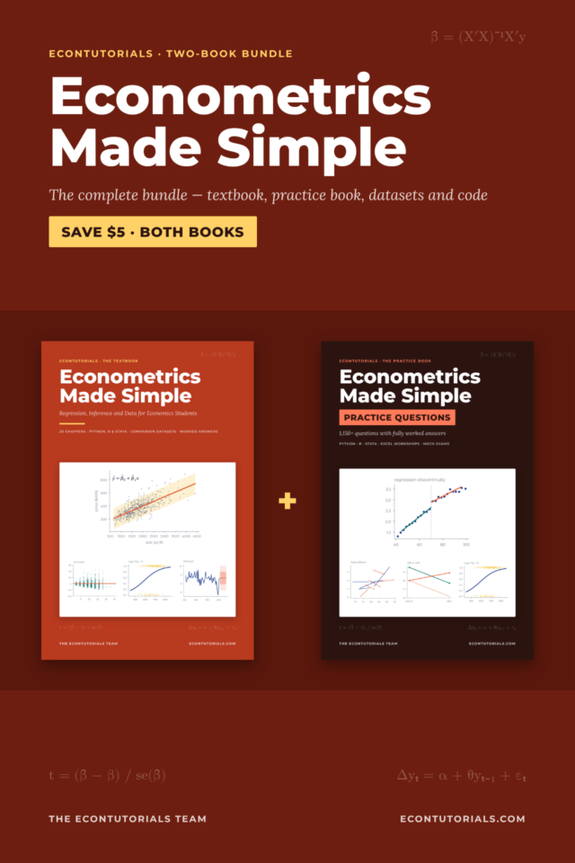
The Econometrics Made Simple textbook builds regression from scratch: what econometrics is (Chapter 1), simple regression and OLS (Chapter 3) and multiple regression (Chapter 6), with Python, R and Stata code. For the statistics groundwork, the Statistics Made Simple Complete Bundle adds the 246-page textbook plus 1,569 practice questions with fully worked answers.
What is Regression Analysis?
Regression analysis is a statistical technique used to examine and quantify the relationship between variables. In economics and econometrics, it allows us to move beyond describing a relationship in words and instead estimate it precisely: by how much does the dependent variable change when an independent variable changes by one unit?
Regression Analysis is a statistical technique that explains the change in a dependent variable due to movement in one or more independent variables. It is a technique for predicting the unknown value of a variable based on the known values of other variables.
Dependent and Independent Variables
Every regression model has:
- Dependent variable (Y) — the variable we are trying to explain or predict. Also called the regressand, explained variable, or response variable.
- Independent variable(s) (X) — the variables we use to explain Y. Also called regressors, explanatory variables, or predictor variables.
Example: Suppose we want to explain the quantity demanded of a good:
Q = f(P, Ps, Yd)
Where Q (quantity demanded) is the dependent variable, and P (price), Ps (price of substitutes), and Yd (income) are the independent variables. Changes in P, Ps, or Yd cause changes in Q.
Important distinction: Regression analysis measures the strength and direction of a relationship, and tests whether it is statistically significant. It does not automatically prove causation — a strong statistical relationship could still be spurious if the theory underlying it is weak.
The Simple Linear Regression Model
The simple regression model involves just one independent variable and takes the form:
Y = β0 + β1X + ε
Where:
- Y = the dependent variable
- X = the independent variable
- β0 = the intercept — the expected value of Y when X = 0
- β1 = the slope coefficient — the change in Y for a one-unit increase in X (ceteris paribus)
- ε (epsilon) = the error term — captures all other factors affecting Y that are not included in the model
Why is it called “linear”?
The model is linear in two senses:
- If plotted, the relationship between Y and X is a straight line.
- It is linear in the parameters (β0 and β1) — this is the more technically precise meaning in econometrics.
 Chapter 3 of Econometrics Made Simple fits a simple regression by hand and then on a house-price dataset, step by step.Get the textbook · $15
The Multiple Regression Model
Most economic phenomena are influenced by more than one variable. The multiple regression model extends the simple model to include several independent variables:
Y = β0 + β1X1 + β2X2 + … + βkXk + ε
Each coefficient βi measures the effect of Xi on Y, holding all other variables constant (ceteris paribus). This is the power of multiple regression — it allows us to isolate the individual effect of each variable.
Example: Wage Equation
Wage = β0 + β1(Education) + β2(Experience) + β3(Female) + ε
Here β1 tells us how much wages increase with an extra year of education, holding experience and gender constant. β3 on the Female dummy variable measures the wage gap between female and male workers with equal education and experience.
Ordinary Least Squares (OLS) Estimation
The most common method for estimating regression coefficients is Ordinary Least Squares (OLS). OLS finds the values of β0 and β1 that minimise the sum of squared residuals — the sum of squared differences between observed Y values and the values predicted by the regression line.
Minimise: Σ(Yi − Ŷi)²
Where Ŷi is the predicted value of Y for observation i. OLS is the Best Linear Unbiased Estimator (BLUE) when the classical regression assumptions are satisfied (Gauss-Markov theorem).
 Make regression second nature: the Practice Questions book starts with the basics and every question has a worked answer.Get 1,150+ questions · $9
Key Regression Output Explained
| Statistic | What it tells you |
|---|---|
| Coefficient (β̂) | The estimated effect of X on Y, ceteris paribus |
| t-statistic | Tests whether the coefficient is statistically significantly different from zero |
| p-value | The probability of getting an estimate at least this far from zero if the true coefficient were zero; p < 0.05 is the usual threshold for significance at 5% |
| R² (R-squared) | The proportion of variation in Y explained by the model; ranges from 0 to 1 |
| Adjusted R² | R² adjusted for the number of predictors; more reliable for comparing models |
| F-statistic | Tests whether the overall model is statistically significant |
Classical Assumptions of OLS
For OLS estimates to be unbiased and efficient, and for the usual tests to be valid, several assumptions must hold:
- The relationship between Y and X is linear in parameters
- No perfect multicollinearity among independent variables
- The error term has zero conditional mean: E(ε | X) = 0 — the factors left in the error are unrelated to the regressors. This is the assumption that makes OLS unbiased; omitted variables that are correlated with X break it
- Homoscedasticity: constant variance of the error term across observations
- No autocorrelation: error terms are not correlated with each other
- The error term is normally distributed (needed for exact t and F tests in small samples; in large samples the tests are approximately valid without it)
Violations of these assumptions (e.g., heteroskedasticity, autocorrelation, endogeneity) require corrective techniques such as robust standard errors or instrumental variables. High but imperfect multicollinearity is not a violation: OLS stays unbiased, but standard errors get larger.
Summary
Regression analysis is the cornerstone of econometrics. It allows economists to estimate the quantitative relationship between variables, test economic theories with data, and make predictions. The simple model Y = β0 + β1X + ε provides the foundation, while the multiple regression model extends it to control for many factors simultaneously. OLS is the standard estimation method, and understanding its assumptions and output is essential for any applied economist.
Studying more than one subject? The Complete Book Bundle gives you every Economics, Statistics, Mathematics, Econometrics and Research Methods book from EconTutorials in one download.
 Textbook plus 1,150+ practice questions: get both Econometrics Made Simple books for $19 (was $24).Both books · $19