To understand regression analysis with dummy variables, let us take an example of using dummy variable with structural changes in an economy. For example, there was a structural change in U.S during 1981-1982, and also a severe recession in 2007 and 2008. So when we taking a time series data, such structural changes does has an effect on our regression analysis. To check the effects of such structural changes, we use a particular dummy variable and then run our regression.
I am taking an example of the economy of Pakistan which had a structural change in 1993 Monetary policy. The data starts from 1976 to 2015. Source of the data is from State bank of Pakistan Statistical handbook.
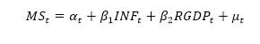
Dummy model equation
To understand the structural changes of the economy we first have to create our model of dependent and independent variables.We know that the overall effect of the independent variable of CPI and Real GDP would cause an effect over the Money Supply (Broad Money, M2) of the Economy. Thus, we can write the equation in the following way:
 Data collection source
To understand the structural change in the Economy of Pakistan we take a time-series data from 1976 to 2015. The source of the data is from Handbook of Statistics of Pakistan Economy from State Bank of Pakistan. For the above equation the following data was collected:
- MS= Board Money M2 from 1976 to 2015
- Inflation = CPI indices – Average general value is taken from 1976 to 2015
- RGDP= Growth rate of the Economy from 1976 to 2015
Log-log, Double log model usage
We will be using double-log at both ends of the equation. Econometricians use natural log for various reasons in regression analysis. The important reasons for taking a double log at both ends for this equation is as follows:
![]()
- It makes a nonlinear equation to linear so that we are able to run the regression analysis.
- It is easier to figure out the impacts in percentage terms.
- In a time series data, we need a natural log to remove the time trends of exponential growth or recession etc.
- It normally distributes a skewed data which is one of the assumptions of classical Linear Regression models that have to be followed.
- Additionally, we take Log of CPI indices to change the commodity prices into inflation rate. (Note that if we want to focus on prices than we should not take a log. Since our model requires inflation rate so we have to run a natural log)
Regression Results of Double-Log Equation
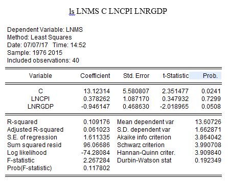
The following command was written in Eview 9.5 student lite version for run the regression of our equation
Interpretation of the result
The result shows that the P values are quiet high, which leads us to the analysis that the CPI is insignificant. (No relationship between Inflation Rate and Money Supply of Board Money in Pakistan)
With regard to the Independent variable of RGDP, it shows us that 1% increase in real GDP would lead to a decrease of -0.9% in MS. The p-value for this coefficient is significant enough which shows there is a strong relationship between Real GDP and MS. (5%). Let us add a structural change dummy variable to understand the exact effects.
Adding the structural change dummy variable (Differential Intercept dummy)
To understand the structural change of 1993 in the economy of Pakistan. We add a differential intercept dummy variable of MP93 in the equation. Note that we don’t take a log of Dummy variable in the equation. Because a dummy variable is coded with 0 and 1 and a log of Zero are considered Undefined (value missing). And the log of one is zero. So when we run a regression of a log dummy, the 0 observations in the dummy are omitted, and the rest of remaining observation with value 1 becomes Zero. Which as a result makes it collinear with the constant in the equation. Hence we don’t take a log of Dummy variable of Structural change of 1993 in our model.
![]()
Where Monetary Policy dummy variable value is 0 from 1976 to 1002 and the value is 1 from 1993 to 2015
Regression with Dummy variable
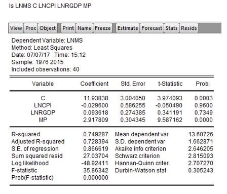
Interpretation of Dummy variable
For the Coefficient of Real GDP, we can interpret that a 1% increase in the RGDP would lead to a 0.09% of Increase in the Money Supply (Board Money-Dependent variable).
However in the case of the Inflation rate, the board money supply of M2 decreases at a rate of 0.02% if the Inflation rate increase by 1%. The p-value for this relationship is very weak (96%)
The structural change of 1993 of monetary policy is about 2.91 which is statistically significant this shows us that there have been changes in Money supply in pre and post-1993.
The R2 value of 72% and an Adjusted R value of 74% shows how well the independent variables of Inflation and Real GDP has explained the model. So higher R values show regression with a good fit. (Note that we always get a high R2 in a time series data because of the significant trends within the observations. Whereas in a cross-sectional data we get a low R2.
Thus, the inclusion of the dummy variable of Structural change of Monetary Policy of 1993 in the regression, show highly significant p-value, which leads us to the analysis that there have been structural changes in the economy.
The forecast for the result is as follows:
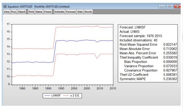
The forecast clearly shows the structural change of the intercept dummy variable of 1993 in the equation.


959750 556833The posh distributed could be described as distinctive; customers are in fact yearning for bags is a Native aspirations. Which strange surroundings is built that is to market diversity furthermore importance with travel and leisure market trends. hotels special offers 618755
823372 524124This internet site is often a walk-through like the information you wanted in regards to this and didnt know who to question. Glimpse here, and you will definitely discover it. 113439
648348 641129Gems form the internet […]very few websites that happen to be detailed below, from our point of view are undoubtedly effectively worth checking out[…] 257320
638867 735652Hello! I could have sworn Ive been to this site before but following browsing through some with the post I realized it is new to me. Nonetheless, Im certainly pleased I identified it and Ill be book-marking and checking back often! 618313
735212 866494hello i discovered your post and thought it was very informational likewise i suggest this site about repairing lap tops Click Here 993705
60904 157334Considerably, the story is in reality the greatest on this noteworthy topic. I agree along with your conclusions and will eagerly watch forward to your next updates. Saying nice one will not just be sufficient, for the fantastic clarity in your writing. I will immediately grab your rss feed to stay privy of any updates! 284761