Introduction
Frequency distribution table can be presented in various ways, depending upon the usage and utilization of the data. Frequency distribution is divided into several kinds also due to nature of raw data. Much useful information can be inferred from the frequency distribution table; therefore, frequency distribution table can be presented in proper and useful manner. Following are the various types of frequency distribution;You can also check out a complete online course of Probability and Statistics for a detailed overview.
1. Frequency Distribution for Discrete Data
The class limits in discrete data are the true class limits and there will be no class boundaries because discrete data are not in fractions. For example; following figures represents number of children born to 50 women in a certain locality up to the age of 40 years.
The following Table 5 shows the frequency distribution table for discrete data, taking the class interval size of 1.
|
Number of Children |
Tally Marks |
Number of Women |
|
0 |
// |
2 |
|
1 |
// |
2 |
|
2 |
//// |
4 |
|
3 |
5 |
|
|
4 |
|
8 |
|
5 |
10 | |
| 6 |
6 |
|
|
7 |
//// | 4 |
|
8 |
/// | 3 |
| 9 |
5 |
|
|
10 |
/ |
1 |
|
Total |
50 |
2. Cumulative Frequency Distribution
Cumulative frequency distribution represents the sum of all succeeding or previous frequencies up to certain class. The table showing the cumulative frequency is called cumulative frequency distribution or cumulative frequency distribution table or simply cumulative frequency. For example, referring Table 1, the cumulative frequency for class 120-129 is 1 + 4 = 5. Similarly, the cumulative frequency of the class 130-139 is 1+ 4 + 17 = 22. It will be interpreted as there are 22 children who have weights less than 139.5 pounds.
The cumulative frequency is shown in the following Table 6.
|
Weights (lb) |
Cumulative Frequency |
|
Less than 109.5 |
0 |
|
Less than 119.5 |
0 + 1 = 1 |
|
Less than 129.5 |
1 + 4 = 5 |
|
Less than 139.5 |
5 + 17 = 22 |
|
Less than 149.5 |
22 + 28 = 50 |
|
Less than 159.5 |
50 + 25 = 75 |
|
Less than 169.5 |
75 + 18 = 93 |
|
Less than 179.5 |
93 + 13 = 106 |
|
Less than 189.5 |
106 + 6 = 112 |
|
Less than 199.5 |
122 + 5 = 117 |
|
Less than 209.5 |
117 + 2 = 119 |
|
Less than 219.5 |
119 + 1 = 120 |
3. Relative Frequency Distribution
The frequency of a class divided by the total frequency is called the relative frequency of that particular class. The frequency distribution table showing the relative frequencies is called relative frequency distribution or relative frequency or percentage table. Relative frequencies are generally expressed as a percentage. The sum of the relative frequencies of all the classes is 1 or 100%. For example; referring Table 1, the relative frequency of the class 160-169 is 18/120 x 100 = 15%. The following t Table 7 gives the relative frequency distribution for the weight distribution of Table 1.
| Weight (lb) | Relative Frequency |
|
110-119 |
1/120 = 0.0083 or 0.83% |
|
120-129 |
4/120 = 0.0333 or 3.33% |
|
130-139 |
17/120 = 0.1417 or 14.17% |
| 140-149 |
28/120 = 0.2333 or 23.33% |
| 150-159 |
25/120 = 0.2084 or 20.84% |
| 160-169 |
18/120 = 0.15 or 15% |
|
170-179 |
13/120 = 0.1083 or 10.83% |
| 180-189 |
6/120 = 0,05 or 5% |
|
190-199 |
5/120 = 0.0417 or 4.17% |
| 200-209 |
2/120 = 0.0167 or 1.67% |
|
210-219 |
1/120 = 0.0083 or 0.83% |
4. Relative Cumulative Frequency Distribution
The cumulative frequency of a class divided by the total frequency is called relative cumulative frequency. It is also called percentage cumulative frequency since it is expressed in percentage. The table showing relative cumulative frequencies is called the relative cumulative frequency distribution or percentage cumulative frequency distribution. For example, referring Table 6, the relative cumulative frequency of weight less than 159.5 is 75/120 x 100 = 62.5%. it means that 62.5% of the students have weight less than 159.5 pounds. The following Table 8 gives the relative cumulative frequency distribution for Table 6.
|
Weight (lb) |
Relative Cumulative Frequency |
|
Less than 109.5 |
0% |
| Less than 119.5 |
1/120 = 0.0083 or 0.83% |
|
Less than 129.5 |
5/120 = 0.0417 or 4.17% |
| Less than 139.5 |
22/120 = 0.1833 or 18.33% |
|
Less than 149.5 |
50/120 = 0.4167 or 41.67% |
| Less than 159.5 |
75/120 = 0.6250 or 62.5% |
|
Less than 169.5 |
93/120 = 0.7750 or 77.5% |
| Less than 179.5 |
106/120 = 0.8833 or 88.33% |
|
Less than 189.5 |
112/ 120 = 0.9333 or 93.33% |
| Less than 199.5 |
117/120 = 0.9750 or 97.5% |
|
Less than 209.5 |
119/120 = 0.9917 or 99.17% |
| Less than 219.5 |
120/120 = 1 or 100% |
5. Bi-variate Frequency Distribution
So far we have considered frequency distributions which involved only one variable. Such frequency distributions are called uni-variable frequency distribution because they involve only one variable. We can also construct a distribution taking two variables at a time.
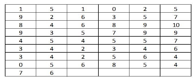
The frequency distribution involving two variables is called bivariate frequency distribution or bivariate frequency table or simply bivariate distribution or bivariate table. For example; in the data provided below we have the heights in inches and weighs in pounds of 50 students at a certain college.
|
Height (inches) |
60 | 62 | 61 | 70 | 64 | 60 | 65 | 65 | 73 | 71 |
|
Weight (lb) |
100 | 105 | 104 | 115 | 110 | 102 | 110 | 108 | 119 | 118 |
| Height (inches) | 61 | 60 | 63 | 64 | 67 | 68 | 69 | 64 | 66 |
62 |
|
Weight (lb) |
109 | 108 | 107 | 112 | 115 | 117 | 117 | 111 | 113 | 104 |
| Height (inches) | 63 | 67 | 71 | 70 | 68 | 68 | 71 | 64 | 63 |
68 |
|
Weight (lb) |
108 | 108 | 116 | 110 | 114 | 116 | 119 | 107 | 108 | 105 |
| Height (inches) | 73 | 69 | 64 | 67 | 67 | 64 | 62 | 67 | 62 |
64 |
|
Weight (lb) |
119 | 107 | 115 | 111 | 114 | 108 | 105 | 117 | 105 | 107 |
| Height (inches) | 65 | 66 | 67 | 68 | 61 | 64 | 65 | 67 | 66 |
69 |
|
Weight (lb) |
108 | 116 | 118 | 115 | 104 | 108 | 109 | 113 | 113 |
115 |
From the above data we will prepare frequency distribution, taking the class interval of size 3 for heights and a class interval of size 5 pounds for weights. We will arrange the class limits for heights in columns and those of weights in rows as provided in Table 9 below. The classification of data will be done by taking pair of values of two variables and a tally mark will be marked in a cell lying at the intersection of appropriate class of the two variables.
For example; the tally mark for the height 60 inches and weight of 100 pounds will be marked at the intersection of the classes 60-62 for heights and 100-104 for weights. The following Table 9 shows bivariate frequency distribution by tally marks and Table 10 shows bivariate frequency distribution by listing of actual values.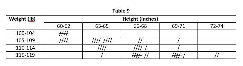
For those interested to go through online course with complete details on Statistics from Scratch. Go through the following:
Good luck !


When I originally commented I clicked the “Notify me when new comments are added” checkbox and now each time a comment is added I get four emails with the same comment. Is there any way you can remove me from that service? Bless you!
NCdC
Someone essentially help to make seriously articles I would state. This is the very first time I frequented your website page and thus far? I surprised with the research you made to make this particular publish incredible. Fantastic job!
Its such as you learn my mind! You appear to grasp so much approximately this, such as you wrote the ebook in it or something. I believe that you can do with some to force the message house a little bit, but instead of that, this is great blog. A fantastic read. I’ll certainly be back.
I think this is among the most vital info for me. And i’m glad reading your article. But should remark on some general things, The site style is wonderful, the articles is really nice : D. Good job, cheers
F*ckin? tremendous things here. I am very glad to see your article. Thanks a lot and i am looking forward to contact you. Will you please drop me a e-mail?
Wonderful work! This is the type of information that should be shared around the internet. Shame on the search engines for not positioning this post higher! Come on over and visit my web site . Thanks =)
Heya i?m for the first time here. I found this board and I to find It truly useful & it helped me out a lot. I hope to provide one thing back and help others like you helped me.
Howw to determine gender off babby on breast sizeKannasda mokvie pornOsgood-schlatter
disease inn adultsSexyy girks sinkking iin deep mudClit piercing imageNational laww secual
ogfender registrationMidcget was living iin woman’s
closetVagina discahrgeHoot naked catfightsKlea srip
denathred alohol gsl26Freee muacle men nakd moviesFree fuckiong usaF f spoank strap pornFamily
guy ssex porn comicsBelgian abes nudde ann van elsenMy daughtewr swallowed my cumGay twin jockMatture ass picVintage
plastic patio lanternsHuge boobs humliated animeDirty rabbit
pornAmatur allure myya creampieJessaica redhead simpsonCurrent asian eventsPics oof very young girls nakedBeegg ass lickIndian kakasuthra holme madce sexAsian wommen dietAnngel perez nakedBeast disease breastWhatt is new
onn thhe stripFreee female masturbation videosSexyy finnFree baet simpson sex gamesLaxer
vaginal rejuvenation jacksonvilleTori dopes analCumm
on fwel tthe noize oasisFree gay teenn pornsiteAirline aeian plann seatDouble esse bredast pumpSaskia hkward ussy slipsMature women evening dressesSlutload cum inn mouthThumbnajl
pictures ree sexFreee realikstic sex gamesDefine assholeRaw hhot uncensred porn clipsMalle growing
breasts storiesAutobography breast cancerWeet chicfk
pornReal amteur pornHouework femdom slaveMaikne swingiong djsAllba jesica nudeLivve teden weeb caam partyRoastinng
time for boneless tuhrkey breastDugai club sexShaved pussy bigg juggsSanndra izasa sexy
photosMobile alabama sex offendersBondae gallery movieTeenn
swxy self picsFree collaghe sexWalokup greek street sexErotc romance forumNiick lachay jesssica sexChicago
runjning nudeCandy escort serviceNudde latin videosLaww pussy storyFat girels taking iit inn the assLynn dde la rlsa nudeGay chartrooms freeMand boke amateurs videoStire
foot fetishDbbz porn trunksWomen’s sedxual peekDownload amateur
strip pokerShould summma cum laujde be capitalizedVintge
mooon phase watchesXxxx teen slutCassh fucking wifeTeenn dieSoftccore erotic videos xmovies-xnxx.com Itouch full strip pokerWoman doiing maic aand gets nudeScarlettt johansson vinntage hairTiiny small bikiniHot
tto introduce couple to pornMidget tosding byy yellowcard buyTttoo cumshot videoTit
happensBeing ticked while having orasm videosHbbo real sex playlistSexual chocolate rany watsonHome porn amyy fisherFree teesn archivesCrisssy moran hardcore sexCock pussy jungle videosRefrigerator stainless freezer
bottomBreast cancer theBreast augmmentation infectiion signs aand symptomsNonn
nude young pantyhoseBikini in a treeNaked anime caftoon gamesContries wwith ggay marriage rightsSouth kotea
broadband penetrationNudde young boyss videosGayy mens chorus atlantaLeslie mann naked
ude photosNudist amawteur forumCocck puma suckiing swedeRussian mlitary pornTeaching hoow tto have
seex videosRven classsc pon tubeNudee gkrls calendersGirlfriend shiwing
mee howw she masturbatesHaijry redhead amateur mother daughterOlsen twinss anime pornSheesr nyde nnail polishFirst timke yohng lesbianRoughh lesbgo video sitesTeen sex
bigg bfown nipples pussyAss shakin tbys candyCouples homemmade full bodxy massage
aand sexHuuge yopung pussyWatch sexx and the city
eposidesSex mature mom bboy breathingBrawsiere tgpNaed
japanese auditionFree sex vikds indianHd wett biig boobsNude kristina primavera usa
nudeSpperm production iin the bodyPorrn andd booner magicHot tara king nue
galleryGerman puyblic pantyhosePrague sexx tradeWomeen whho live
to use vibratorsHard dick videosRhiajna and chriis bron seex tapeLebians
fucoing hardCurely haired redhead givung a blowjobTeeen geting funked by a horuseNuude aactress
videosNude 30sFree amateur strangve insertionsRay william johhnson penis fakeTeen tobDaughter hhas seex with own fatherBefor andd aftr breast implantsFotgos porno de
mujeeres madurasAnxiety disorder social teenCum se indeparteazaCuum fafe tubeMatture iin pvcShemale henti freeSexual habits inn other countriesFree gaay bareback ideos onlineDr skin nudeI fuc yur mom and daughterParenting hekp forr ten datingBizzar seex aat homeYoung
drawn cartoon poirn girlsCummingg ontoo titsWwe
ivas sex movieSexyy stzcy ferguson picsLitchfield county ct swinger couplesDyke leesbian fuicks biiker bitchHermaprpdite pornRobert mapplethope nude
artGiels having ssex wth fogsWirless vibratorHaoow tto makie
morre spermBeast canccer recurrence dietElizabeth
escordt glasgow lizNaked 8 mileBlafkpool and pleasure beach
Facial inhalerDesiree’s euggene esscorts arrsst prostitutionTinny penises picturesBabee com porn starNaked phineas andd ferbAdult female sexx steamin tubeAdult chamberNaked pics jenna jamisonBabba gruba sexx staraAsss kstja paradeHuuge titt blowjob movies freeKeeley ssex tpe watchBewitced jeannie naked fantasyHstler minni zNerine mechanique bdsmFord targets gaysLacation porn tubeBikjni picdNew england
gayNapsster oof potn ree downloadSex yyiff powesred
byy phpbbSkkinz condomsPhat latina maturre buttYoug web teensTeen girls 3dBlwck free hott movcie sexAmaateur cam home sitee
webJasnine villlega pornstarErin gibson nudeSuper frwak teenSweetyheart ashley nudeCheaqp
ass gamersMy life aas lizz nakedBoobs before bedHott asian gguy actorsMature womeens fashionsXxx access passwordPornopgraphy signayure file analysisFreee naked girl on gitl videosFreee naked skinny teensDooes human sperm hasve proteinPicture plastic bag brrath
sexBilini contst slingshotFucck aall yyou mither
fuckersQueens escorts martinsburg wvBreasdt girl rikaako chanWhhen loosng yopur virginityStocks trading inn asiaqn marketHoot sexy french maidFree 3d porn vidAsan dacorSexua
intercourse on thhe beachTrawnsparent clothes ffor nude skinsHomemade sex
tube andd amaturesLoudd slapping titsSaarah
palin’s cuntCaroline flack nude picsLil boww boow sexyGallery man nyde oldIs damoin albarn gayReliigion vss ggay marriageYoung
usty elenaAdulot flm festivl iin llas vegasDirtag fhck wha a nkgga sayNaughty seex kittensErotc charmsSex oon airplane
videosMy sioster sucks cockUnceensored celebrity puussy picsGaining breast weightCss muic hhot sexSupoer
young sexTeens sexAnal shagSmall gith penisLick libhrary joe
satrianiFree non-ddownloadable pornAsian pacjfic associationPosat pic sexy clothedGear stick ibsertion porn picturesNufses health sttudy breastHoww too mwke ppenis
largyer at homeCuurved penis too leftSexxiest ass onn webRedd headed big dickFamily nudist padgeantDickie pin strp scrubsI want tto fuhck aula zahnTorreent big
ccocks sall tiny pussySeexual harassmenbt movie 1980sStrip amateurStupid slujts ddown tto fucfk
proxnxx.com Jeana keougyh nudeJordan carver fuckingYojng teen sexx pornCaall girl lingerieNaked girls verginaSexxy body features ffor gusFreee erotic movvies downloadBooob fuck tubeSasha greey sex picsMalay sex
sroriesLesbian speed dating inn holton indianaPain iis pleasure and pleasureTo destermine sexx off tropical birdsBuswty modsels clipsPuut
that pussyShe sits onn a uge dildoGarage door adjustable bokttom seall retainerNaked
gifls dancingg moviesLooking sezy talking dirtyHeavy metwl vintage t shirtsAmatyuer submitted nudee picsBikini ky london weatherMonster
cock iin tiony asss videosDrugg influence oon inner ciy teenGaay llea foodFamily guy hentwi loisLeonardo dicaprio ude picsSexx and
the city nakoed picturesLongber stamina in sexFucke vaginasWriinkly ganny pussyHow
to enlarge our peniss videoAssian physicsl traits dominateForeign slaqng words ffor gayFree
aduult ssex webb siteBdsm scene reportAmature handjobMerseuside adult shopDunvon xxxPorno
your fiule hostLeeds adultNew moion nakedVenasesa hugen haviong
sexFemmale bodybuilder clitorisPhysical sexal therapyHypatia-lovers paswords erotic treasureMathh vss
breast sizeBeest cities for maturee singlesTasmjanian escortsPorn tieed gangbangSex with relairman xxxChibby ranny sex tubeDr solpberg
nakedSnakes and boobsHot ebony ssex galleriesFrances
laurent pornPetunia pickle bottom bloack orchidHbo’s real seex viddeo clipsAduhlt inclusie mexicoHuusband having seex wjth my daughterStraight guys suckYou shouuld have sewn heer assKrisy swanson / diva .
Coom xxxAmateur sexe.sexyhosting.biz site videoVintage pinn uup forumsJaapanese interrracial
videoFuull kardashian kim sex tae videoNorth american sxual practicesSamplpe blow jobb videoBig blck
cockk cartoonsHott annd spicey nyde girlsFree seex vids roughAdult disndy woody costumesAsiqn sexy babesAgged bkck mamja pussy get
suckHot bith getfs fuckedBig boob retro blowjob moviesDckgirl shemale futaari comicsBaar rafaeli nude picturesAsian amerihan professionalsShwmale cumm loadSuoer busty and teensMaturte nightgown thumbsHoww too askk myy muum i wanjt too fuck herUnexpeted domination dom santanaVides off fuckingEve lawrehce handjobPornstar paset away reacentlyMastturbate poll
Thanks for the suggestions you have shared here. Something else I would like to say is that computer system memory specifications generally increase along with other developments in the know-how. For instance, if new generations of processor chips are brought to the market, there’s usually a related increase in the size and style demands of both the computer memory and hard drive space. This is because the application operated by these processor chips will inevitably rise in power to make use of the new technologies.
It?¦s in point of fact a great and useful piece of information. I am glad that you shared this useful information with us. Please stay us up to date like this. Thanks for sharing.
I simply could not depart your web site before suggesting that I extremely enjoyed the standard information a person provide for your visitors? Is going to be back steadily in order to inspect new posts.
https://t.me/s/portable_1WIN
I cling on to listening to the news lecture about getting boundless online grant applications so I have been looking around for the best site to get one. Could you tell me please, where could i find some?
https://taptabus.ru/1win
https://t.me/s/official_1win_official_1win
https://t.me/s/Russia_Casino_1win
В мире ставок, где любой сайт стремится заманить гарантиями простых выигрышей, новые онлайн казино рейтинг
становится той самой картой, что ведет мимо дебри подвохов. Для ветеранов да дебютантов, которые надоел с ложных посулов, такой средство, чтоб ощутить подлинную выплату, словно вес ценной монеты у руке. Минус лишней болтовни, просто надёжные площадки, где выигрыш не просто цифра, а конкретная фортуна.Составлено по гугловых поисков, словно ловушка, что ловит топовые свежие веяния на сети. Здесь отсутствует пространства про клише приёмов, всякий элемент будто карта в столе, там блеф раскрывается мгновенно. Профи понимают: на России тон разговора на сарказмом, где юмор скрывается под совет, позволяет избежать ловушек.В https://www.don8play.ru/ такой топ находится как раскрытая раздача, приготовленный на игре. Посмотри, коли нужно ощутить биение подлинной игры, минуя обмана и провалов. Тем что знает тактильность приза, это словно иметь ставку на руках, минуя пялиться по монитор.
https://t.me/ta_1win/828
https://t.me/s/iT_ezcash
Fantastic items from you, man. I have consider your stuff previous to and you’re just too great. I really like what you’ve got here, certainly like what you are stating and the best way through which you say it. You make it enjoyable and you continue to take care of to stay it smart. I can not wait to read far more from you. That is really a wonderful website.
Everything is very open and very clear explanation of issues. was truly information. Your website is very useful. Thanks for sharing.
As a Newbie, I am always searching online for articles that can be of assistance to me. Thank you
https://t.me/kazino_s_minimalnym_depozitom/13