Introduction

Before preparing frequency distribution it is necessary to collect data of the required nature from the various sources. The data collected is always in raw form which is needed to be arranged in a proper arrangement for the purpose of inferring the required results. You need to do certain preparations for frequency distribution, which includes the classification and tabulation of data. Both of them are explained in detail as follows;

Classification

“The process of arranging data into classes or categories according to some common characteristics present in the data is called classification”

Collected data are usually available in a form which is not easy to comprehend. For  example, if we have before us the marks obtained by 1000 universities students at their Undergraduate Examination, it would be difficult to tell simply by looking at the marks as to how many students have marks between 300 and 400, between 400 and 500, and so on. In order to get the clear picture of the situation, the data must be present in a manner which is easy to understand. As first step, we arrange the data into classes and categories having similar characteristics. For example, we may arrange the marks into groups of 50 marks each, e.g. 300 t0 349, 350 to 399, 400 to 449 and so on.

Basis for Classification

The collected data can be classified by many characteristics, there are four main basis of classification are mostly being practiced. These bases are;

1. Qualitative

• When data are classified by attributes, e.g. religion, marital status etc.2.

2. Quantitative:

• When data are classified by quantitative characteristics, e.g. height, weight, income, etc.

3. Geographical:

• When data are classified by geographical regions or locations, e.g. the population of a country may be classified by provinces, divisions, districts or towns.

4. Chronological/Temporal:

When data are classified by their time of occurrence. An arrangement of data by their time of occurrence is called a time series.

Tabulation

“The process of arranging data into rows and columns is called tabulation”

A table is a systematic arrangement of data into vertical column and horizontal rows. Tabulation of data on population of a country can by classified on the basis of religion, gender or marital status. Tabulation may be simple, double, triple or complex depending on the nature of classification, which is being used by the statistician.

Frequency Distribution

“A frequency distribution is a tabular arrangement of data in which various items are arranged into classes and the number of items falling in each class is being mentioned”

We have discussed the classification and tabulation of data. Frequency distribution is an important method of summarizing and organizing quantitative data. The data which is presented in the form of frequency distribution is called grouped data, whereas, the data which has not been arranged in a systematic order or in the form of frequency distribution is called raw data or ungrouped data.

For Example

Let us consider the weight of 120 students at a university, as given below;

 

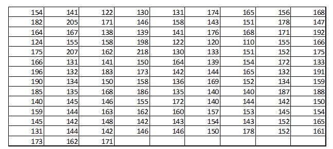
From the above provided data it is difficult to draw any meaningful conclusions. As in, it is difficult to tell simply by looking at the above data as to how many students have weights below or above 150 pounds or between 150 and 200 pounds and so on. Therefore, necessary to arrange the data in such a way as their main features as clear. Conclusion can easily be drawn if the data is arranged in an array. An arrangement of data in ascending or descending order is called an array.

From the array many question regarding the data could be answered. But still it will be difficult to look at 120 observations and obtain an accurate idea as to how these observations are distributed. Therefore, we can arrange them in better form. For example, the data may be arranged into classes as shown in following Table 1.

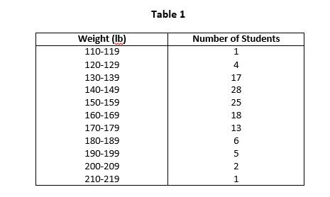
By arranging the raw data in the above form we have distributed the data into classes and determined the number of items belonging to each class i.e. class frequency. The range of data from 110 to 119 is a single class and 1 is it’s corresponding frequency. Such an arrangement of data by classes together with their corresponding class frequencies is called frequency distribution or frequency table.

Class Limits

In Table 1 we see that each class is described by two numbers. These numbers are called class limits. The smaller number is called the lower class limit, and the larger number is called upper class limit. For example, in Table 1, the class limits for first class are 110 and 119. 110 is the lower class limit and 119 is the upper class limit.

Class Boundaries

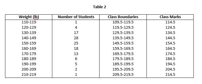
Class limits are not always exactly what they look like. We know that measurements are seldom exact, most of the time they involve approximates and estimations. A weight of 110 pounds means a weight lying between 109.5 and 110.5 pounds. And a weight 119 pounds means a weight lying between 118.5 and 119.5 pounds. When the lower class limit is given as 110 pounds, the true lower class limit is, therefore, the 109.5 pounds and when the upper class limit is given as 119 pounds, the true upper class limit is actually 109.5 pounds. Therefore, if the weights are recorded to the nearest pounds, the class 110-119 includes all the measurements from 109.5 to 119.5 pounds.

The values 109.5 and 119.5 which describe the true class limits of a class are the called the true class limits or class boundaries. The smaller number 109.5 is lower class boundary and the larger number 119.5 is called upper class boundary. Class boundaries are clearly shown in Table 2.

The class boundary can be obtained by adding the upper class limit of one class to the lower class limit of the next higher class and then dividing by 2. Mathematically it can be represented as follows;

For Example, Class boundaries for first class in Table 1 is calculated as;

 The Class Marks or Midpoints

“The class mark or the midpoint is that value which divides a class into two equal parts”

The class mark or midpoint can be obtained by adding the lower class limit and the upper class limit or class boundary of a class and dividing the resulting figure by 2. Mathematically it can represent as follows;

 

For Example, Class mark of the first class in Table 2 below, will be calculated as;

The following Table 2 shows the class boundaries and class marks for the corresponding classes,

Size of Class Interval

“The size of the class interval, which is also called the class width or class length, is the difference between the upper class boundary and the lower class boundary”.

Class interval is not the difference between the class limits. Where all the class intervals of a frequency distribution are of equal size, the common width id denoted by h. In such case, the size of the class interval is also equal to the difference between the two successive lower or upper class limits. For example, in Table 2 the class interval for first class is 119.5 – 109.5 = 10, or 120 – 110 = 10.

Formation of a Frequency Distribution

Following steps are involved in the formation of a frequency distribution:

• Determine the greatest and the smallest number:

First of all determine the greatest and the smallest number in the raw data and find the range, which is the difference between the greatest and the smallest numbers. In the example of weights of 120 students, the greatest number is 218 and the smallest number is 110. Therefore, the range is 218 – 110 =108.

• Decide on the number of class:

For the purpose of determining the classes for the frequency distribution there is no hard and fast rules for the purpose. Mostly, 5 to 20 classes are being made. The number of classes should be appropriate, so that could be distributed and represented properly. If we have less than 5 classes, it will result in too much information being lost. On the other hand, if we have more than 20 classes, computation will become unnecessarily lengthy. In Table 1 we have made 11 classes.

• Determine the approximate class interval size:

The approximate class interval size is determined by dividing the range of the desirable number of classes. For example, in the raw data of weights of 120 students, the class interval size is 108/11 = 9.8 or 10. A number used as class interval size should be easy to work with.

• Decide what should be the lower class limit:

The lower class limit should cover the smallest value in the raw data.

• Find the upper class boundary by adding the class interval size to the lower class boundary:

The upper class boundary of a particular class is determined by adding the class interval size to the lower class boundary of such class. The remaining lower and upper class boundaries are determined by adding the class interval repeatedly until the largest measurement of the raw data is enclosed in the final class.

• Distribute the values of the raw data into classes:

The class frequencies are obtained by distributing the raw data measurements into the classes made. The number of measurements falling in each class is referred as it frequency.

Methods for Frequency Distribution

There are two methods for arranging the observations in their proper classes. Such methods are as follows;

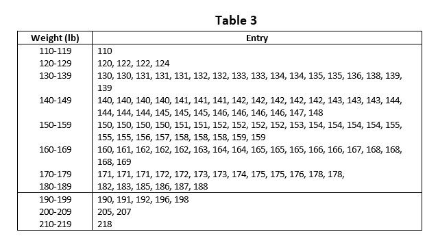
• By Listing the Actual Values:

In this method of frequency distribution, each observation is listed in its proper class. The following Table 3 illustrates the tabulation of weight measurements of 120 students. This is called entry table.

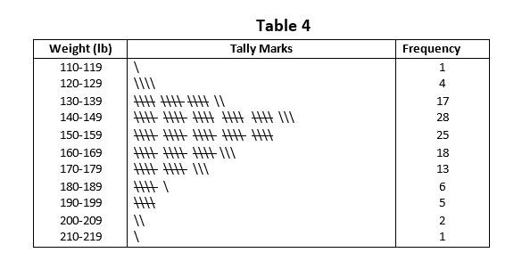
• By Using Tally Marks:

This method of frequency distribution is used where the data are not arranged in order of magnitude. The easiest way of tabulation data is by recording stroke i.e. tally mark, opposite the appropriate class for each observation. The following Table 4 illustrates the frequency distribution by using tally mark.