Monopoly’s Output Decision

The output decisions in case of monopoly differ in respects of the time period or the length of time span through the monopoly firm is operating. There are two kinds of time periods;

i. Short Run: It is a time period in which one of the variable is fixed i.e could not be altered.

ii. Long Run: It is a time period in which all the inputs are variable i.e variables or inputs are changeable.

Short Run Equilibrium

In short run a monopoly firm attains the level of equilibrium when any of the following two conditions are fulfilled;

1. Profits are maximum, or
2. Losses are minimized

When the condition (i) is fulfilled and the profits are being maximized, in order to achieve maximum profit in short run further two conditions are required to be fulfilled;

1. Marginal Cost is equal to Marginal Revenue i.e MC=MR
2. The slope of MC is greater than the slope of MR at the point where both of them intersect.

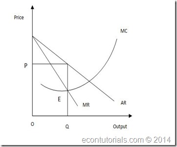
The above is called as Marginal Revenue and Marginal Cost Approach. According to this approach the firm is in equilibrium at the point where MC=MR. This is shown in the following graph:

In the above graph it is clearly visible that MR is intersecting MC curve at equilibrium point E. At point E both of the condition of profit maximization are fulfilled that;

1. MC=MR
2. MC curve intersects MR curve from below.

In short run there are three cases of profits which a monopoly firm can earn. The basic variance in different kinds of profit is usually of the average cost covered by profit. This will be cleared with the help of following explanation of output decisions of monopoly in short run.

Abnormal Profit

The monopoly firm will select such a level where it produces better output which will yield him maximum profit. Such level will be the equilibrium point where marginal revue is equal to marginal cost.

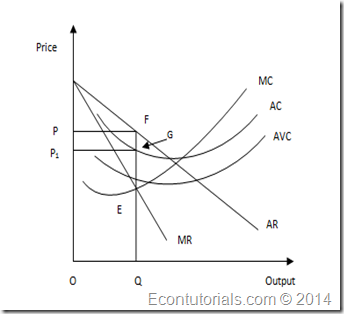
In the above graph the average cost curve (AR) which is also the demand curve for the monopolist. The AR slopes downwards. Below the AR, there is marginal revenue (MR) curve. MC is the marginal cost curve which intersects MR at point e which is the equilibrium point of profit maximization of the monopoly firm. OQ is the total output of the firm. At this level the total revenue of the firm is greater than the total cost of the firm and the firm is earning abnormal profit.

• Equilibrium point = E
• Output = OQ
• Total Cost = TC = OQGP₁
• Total Revenue = TR = OQFP
• Abnormal Profit = TR – TC = FPGP₁

Normal Profit

In case of normal profit the equilibrium point is the point where MC = MR and AC = AR. This can also be explained as that a monopoly firm earns normal profit when total cost of the firm becomes equal to its total revenue.

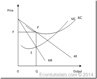
In the above graph the firm is at equilibrium point E and it is producing the output OQ at equilibrium level. Since, the average revenue is equal to average cost, therefore, the firm is earning normal profit.

• Equilibrium point = E
• Output = OQ
• Total Revenue = TR = OQFP
• Total Cost = TC = OQFP
• Normal Profit = TR = TC

Normal Loss

A monopoly firm suffers from normal loss when its average cost is not covered by average revenue. In such case the total cost is greater than total cost. Total cost comprises of variable cost and fixed cost. For monopoly firm the situation of normal loss arises when its variable cost and a small portion of fixed cost is being compensated by total revenue. Whole fixed cost is not being covered. In normal loss the equilibrium level is the point where MC = MR and AC is greater than AR.

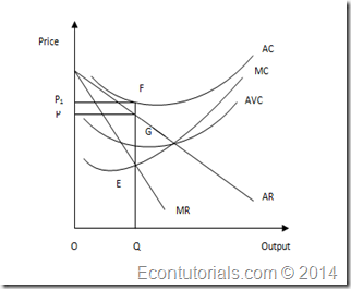
In the above graph it is shown that the monopoly firm is producing at output level OQ where MC = MR. At this point average revenue AR is less than average cost AC. In this situation the whole variable cost and fixed cost is covered, hence, the firm is suffering from normal loss.

• Equilibrium point = E
• Output = OQ
• Total Revenue = TR = OQGP
• Total Cost = TC = OQFP₁
• Normal Loss = TC – TR = PGFP₁

Long Run Equilibrium

In long run the firm has the opportunity to expand its production level by installing new machinery or to upgrade the size of its plant in order to decrease the cost of production or to enjoy the economies of scale, since in long run the costs are variable. Moreover, the monopoly firm is protected by entrance barrier and no competition is faced by it. There could be different kind of entrance barriers in the form of economies of scale which is natural monopoly or in form of legal protection or rights which is termed as legal monopoly.

In such situations the monopoly firm earns abnormal profit. For abnormal profit the average revenue curve AR should be above the long run average cost LAC.

 

In the above graph it is shown that the equilibrium point E is the point where long run marginal cost curve LMC cuts MR. The production of the firm is OQ. And the total revenue is greater than the total cost.

• Equilibrium point = E
• Output = OQ
• Total Revenue = TR = OQJP
• Total Cost = TC = OQKP₁
• Abnormal Profit = TR –TC = P₁KJP

For long run the profit may vary according to capacity utilization of firm under monopoly. There could be three cases;

1. Use of less than Optimal Scale of Plant
2. Use of Optimum Scale of Plant
3. Use of more than Optimum Scale of Plant