Definition

“Regression is a process by which we estimate one of the variables, which is dependent variable, on the basis of another variable, which is independent .”

Dependent Variable

Dependent variable is the one which is intended to be estimate or predicted is referred as dependent variable. Dependent variable is also known as regressand, predicted variable, responsive variable or explained variable. The dependent variable whose values are determined on the basis of the independent variable is called random variable. or

Independent Variable

The variable on the basis of which dependent variable is predicted estimated is called the independent variable. The independent variable is also called regressor, predictor, regression variable or explanatory variable. The values of independent variable are chosen by the experimenter and are assumed to be as fixed.

For Example

If we want to estimate the heights of children on the basis of their ages, than the height will be the dependent variable and age will be the independent variable. Similarly, if we want to calculate yield of crop on the basis of amount of fertilizer used, than the yield will be dependent variable and the amount of fertilizer used will be independent variable.

Explanation

If X is the independent variable and Y is the independent variable, then the relation between the two variables will be described by a straight line. Mathematically, straight line will be represented as follows;

The above equation is called linear equation. It is the usual practice to express relation between the variables in the form of equation. Such an equation connects the two variables. To solve such equation, first of all we need to collect data showing corresponding value of the variables, which will be further be considered for solving the problem. Suppose X and Y denote the respectively the heights and weights of students. Then a sample of n individuals would give the heights as and the corresponding weights will be as.

If Y is to be estimated on the basis of X by means of linear equation, or any other equation, than we shall call the linear equation as the regression equation of Y on X. Whereas, if we intended to estimate X on the basis of Y, than the linear equation shall be called the regression equation of X on Y.When two variables are involved in the process of regression than the process shall be referred as simple regression. If there are three or more variables are involved in the regression process than the process shall be named as multiple regressions.

Properties of Relationship between Two Variables:

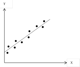
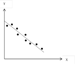
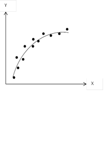
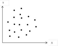
The relationship between two variables is divided into four categories, which as follows;

i. Positive Linear Relationship

Graph 1

ii. Negative Linear Relationship

Graph 2

iii. Non-linear Relationship

Graph 3

iv. No Relationship

Graph 4

Calculation of Regression

The problem of regression is solved by the method of least square. The method of least square is defined as follows;

“Of all the possible cures or lines which can be drawn to approximate a given set of data, the best fitting curve or line is the one for which the sum of squares of deviations, which is the vertical distances between the observed values and the corresponding estimated values, is least.”

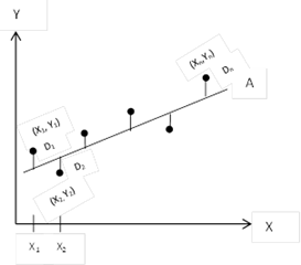
It is the requirement of the least square method that the sum of squares of the vertical deviations, the distances, from the points to the curve or line is minimum. Therefore, if represents the vertical deviations from the points to the line A, as shown in the following Graph 5, then the curve or line has the property that is minimum. Thus a line having this property is called least square line. A curve bearing this property is perfect for the least square sense and is called a least square curve.

Graph 5

In the definition of least squares as provided above, we use Y for the dependent variable and X for the independent variable. Conversely, if X is used as dependent variable and Y is used as independent variable, then the definition of least square provided will be modified and we consider horizontal deviations instead of vertical deviations.

Since the regression is represented by the linear equation, therefore, the equation of least square is also the linear equation. i.e. . The normal equations for regressions are as follows;

………. Eq. (i)

……. Eq. (ii)

Where, a and b are the constants. The above first equation is obtained by multiplying both sides of linear equation by ∑ and then summing both sides of the equation.

i.e.

The second equation is obtained by multiplying the linear equation by X and them summing both sides of the equation.

i.e.

By solving Eq. (i) and (ii) simultaneously we the equations for solving the constants a and b, which are provided below;

Contrary, if the variable X is taken as dependent variable and variable Y is taken independent variable, then the above equation shall be modified. The linear equation or the least square equation will become as;

The normal equations will become as;

And the equations for constants c and d will become as;

For Example:

Find the linear equation . For the following values of X and Y. Find the estimated values of and show that , by using least square method.

X	1	2	3	4	5
Y	2	5	6	8	9

The following Table 20 will be used in solving the problem.

Table 20

X	Y	XY	X2	Y’	D = Y – Y’
1	2	2	1	2.6	-0.6
2	5	10	4	4.3	0.7
3	6	18	9	6	0
4	8	32	16	7.7	0.3
5	9	45	25	9.4	-0.4
∑X = 15	∑Y = 30	∑XY = 107	∑X2 = 55	∑Y’ = 30	∑D = 0

n = 5

Using the normal equations;

Putting the values from Table 2o into the above equations, we will get the following;

To solve the above Eq. 1 and Eq. 2 simultaneously, we will multiply the Eq. 1 by 3 and subtract it from Eq. 2

Substituting the value b in Eq. 2

By solving the equations simultaneously we get a = 0.9 and b = 1.7

Thus the equation of least square line is

For Y’ we put the values of X, given in table, in the least square equation. Like, for X = 1, Y = 0.9 +1.7(1) =2.6, and so on. D stands for deviations. Deviations of Y from the estimated values of Y’ are shown in the Table 20 which are added to give 0.

For Example:

Find the least square line of regression for the following values of X and Y, taking

i. X as independent variable

For obtaining the least square line of regression we will use the following Table 21

Table 21

X	Y	XY	X2	Y2
1	1	1	1	1
3	2	6	9	4
5	5	25	25	25
6	5	30	36	25
7	6	42	49	36
9	7	63	81	49
10	7	70	100	49
13	8	104	169	64
∑X = 54	∑Y = 41	∑XY = 341	∑X2 = 470	∑Y2 = 263

n = 8

We will solve the problem by using the formulas for constant a, b, c and d.

i.

For X as independent variable, the least square line for regression will be

ii.

For Y as independent variable, the least square line of regression is